NumPy gives Python fast, compact, multi-dimensional arrays — the foundation of scientific computing, data analysis and machine learning.
On this page
- What you will learn
- Why NumPy?
- Setup
- Creating arrays
- Array attributes
- Indexing and slicing
- View vs copy
- Element-wise operations
- Sorting, concatenating, transposing, flipping
- Adding and removing elements
- Unique values
- Missing data: NaN
- Saving and loading
- Practical example: production matrices
- Practical example: Punnett squares
- Practice
- Quick reference
- References
What you will learn
By the end of this tutorial you should be able to:
- explain why NumPy exists and when to reach for it instead of plain Python lists,
- create and inspect arrays (
shape,dtype,ndim,size), - index, slice, reshape and combine arrays,
- run arithmetic, statistical and boolean operations efficiently,
- handle missing data (
NaN), - save and load arrays to disk.
NumPy is the backbone of the Python data stack. Pandas, scikit-learn, PyTorch and TensorFlow all rely on it. Time spent here pays back in every data project that follows.
Why NumPy?
Python is easy to read and write, but plain lists are not designed for numerical work. A list of one million numbers can occupy ten times more memory than the equivalent NumPy array, and a loop over a list is much slower than the same operation in NumPy.
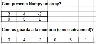
NumPy (short for Numerical Python) solves this with the ndarray — an N-dimensional array stored as a contiguous block of memory of a single data type, with operations implemented in C.
The two key benefits are:
- Less memory. Each element occupies exactly the bytes its type needs (e.g. 2 bytes for
int16), nothing else. - More speed. Operations are vectorised — they run as a single C loop instead of a Python
forloop.
Setup
Create a new project with uv and add NumPy:
uv init numpy-labcd numpy-labuv add numpyOpen a Python REPL inside the project:
uv run pythonBy convention NumPy is imported as np:
import numpy as npEvery example in this tutorial assumes that import is already in place.
Creating arrays
From a Python list
The simplest way is to pass a list to np.array():
a = np.array([1, 2, 3, 4, 5, 6])print(a)# [1 2 3 4 5 6]For a 2D array, pass a list of lists. Each inner list is one row:
b = np.array([[1, 2, 3], [4, 5, 6]])print(b)# [[1 2 3]# [4 5 6]]Type homogeneity
A Python list can hold values of many types. A NumPy array can technically be built the same way, but NumPy will up-cast everything to a single type so the array stays homogeneous:
a = np.array([1, "hello", False])print(a.dtype)# <U21 # Unicode string of up to 21 charactersprint(a)# ['1' 'hello' 'False']If we force a numeric dtype, NumPy refuses the conversion that would lose information:
np.array([1, "hello", False], dtype=int)# ValueError: invalid literal for int() with base 10: 'hello'This is a feature, not a bug — strict typing helps catch dirty data early.
A common mistake when reading data from a CSV: a single text value sneaks into a column of numbers and silently turns the whole array into strings. Any later math then fails with a confusing UFuncNoLoopError. Always check arr.dtype after loading data.
Factory functions
You don’t always have the values up front. NumPy has factories that build arrays of a given shape:
np.zeros(3) # array([0., 0., 0.])np.ones((2, 3)) # 2x3 array filled with 1.0np.full((2, 2), 7) # 2x2 array filled with 7np.eye(3) # 3x3 identity matrixnp.empty() allocates memory without initialising it. It is faster than zeros because it skips the write step, but the contents are whatever was previously in that memory region:
np.empty((2, 3))# array([[ 5.6e-308, 4.0e+00, 9.5e-307], # garbage# [ 8.5e-308, 1.5e-307, 3.5e-308]])Use empty only when you know you will overwrite every element straight after.
Sequences and ranges
np.arange(4) # array([0, 1, 2, 3])np.arange(2, 10, 2) # array([2, 4, 6, 8]) start, stop, stepnp.linspace(0, 1, 5) # array([0. , 0.25, 0.5, 0.75, 1. ])arange is like Python’s range but returns an array. linspace divides an interval into equally spaced points (endpoint included).
Random arrays
The modern way to generate random numbers is via a Generator:
rng = np.random.default_rng(seed=42)rng.integers(low=0, high=10, size=(2, 4))# array([[0, 7, 6, 4],#        [4, 8, 0, 6]])
rng.random((2, 3))   # uniform floats in [0, 1)rng.normal(loc=0, scale=1, size=5)  # samples from N(0, 1)
Pass seed whenever you want reproducible output.
Three patients have their temperature taken on four different days:
| Patient | Day 1 | Day 2 | Day 3 | Day 4 |
|---|---|---|---|---|
| 1 | 39.6 | 38.4 | 36.5 | 36.4 |
| 2 | 39.0 | 38.4 | 37.6 | 37.9 |
| 3 | 37.5 | 37.1 | 36.3 | 36.0 |
Store the data in a NumPy array, then print:
- patient 1’s temperature on day 1,
- all of patient 2’s temperatures,
- every patient’s temperature on day 1.
import numpy as np
temps = np.array([    [39.6, 38.4, 36.5, 36.4],    [39.0, 38.4, 37.6, 37.9],    [37.5, 37.1, 36.3, 36.0],])
print(temps[0, 0])     # 39.6print(temps[1])        # [39.  38.4 37.6 37.9]print(temps[:, 0])     # [39.6 39.  37.5]
Note the difference between temps[1] (row 1) and temps[:, 0] (column 0). The colon : means “every value along this axis”.
Array attributes
Every ndarray carries metadata describing its shape and the values it holds:
| Attribute | Meaning |
|---|---|
ndim | number of dimensions (axes) |
shape | tuple with the size along each dimension |
size | total number of elements (= prod(shape)) |
dtype | type of the elements (int32, float64, …) |
itemsize | bytes occupied by one element |
nbytes | total bytes used (= size * itemsize) |
A picture helps:
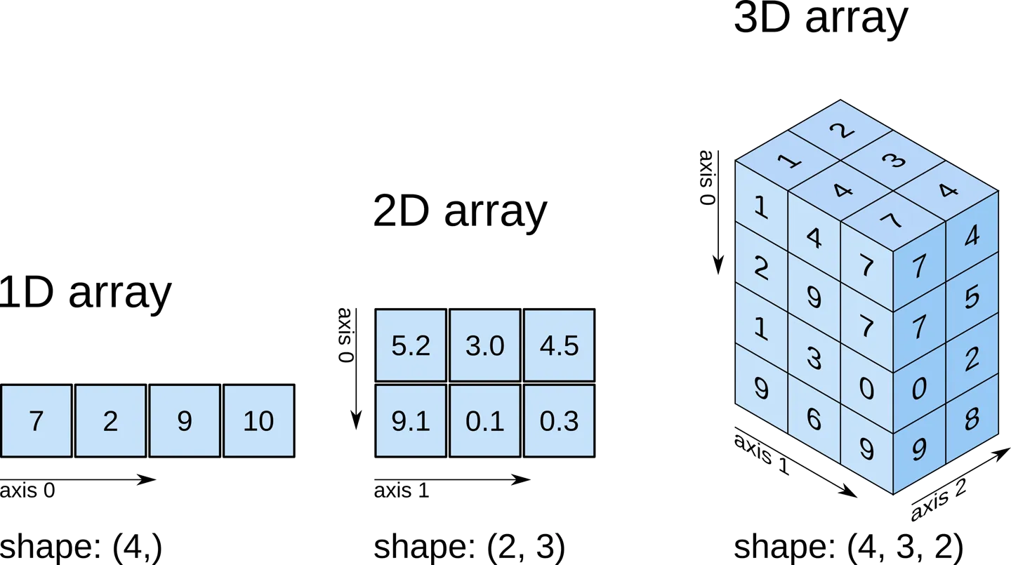
Try it on a 3D array:
a = np.array([    [[0, 1, 2, 3], [4, 5, 6, 7]],    [[0, 1, 2, 3], [4, 5, 6, 7]],    [[0, 1, 2, 3], [4, 5, 6, 7]],])
print(a.ndim)    # 3print(a.shape)   # (3, 2, 4)print(a.size)    # 24print(a.dtype)   # int64
Choosing a dtype
The default integer type is int64 and the default float type is float64 (8 bytes each). For large datasets that is often wasteful — patient temperatures or pixel values fit comfortably in 1 or 2 bytes.
ones64 = np.ones((1000, 1000)) # 8 MBones16 = np.ones((1000, 1000), dtype=np.int16) # 2 MBprint(ones64.nbytes, ones16.nbytes)# 8000000 2000000Dropping from float64 to int16 here saves 75% of the memory. With millions of rows this is the difference between a script that fits in RAM and one that thrashes the swap.
For everyday Python code don’t worry about types — Python integers are unbounded and floats are 64-bit. Only think about dtype once you start handling large arrays.
Indexing and slicing
NumPy uses the same [start:stop:step] syntax as Python lists, but extends it to multiple dimensions.
1D arrays
a = np.array([10, 20, 30, 40, 50])
a[0]      # 10a[-1]     # 50a[1:4]    # array([20, 30, 40])a[::2]    # array([10, 30, 50])  every second elementa[::-1]   # array([50, 40, 30, 20, 10])  reversed
2D arrays
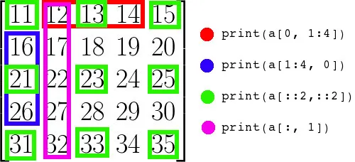
A 2D array uses two indices: a[row, column]. You can replace either with a slice.
a = np.array([    [ 1,  2,  3,  4],    [ 5,  6,  7,  8],    [ 9, 10, 11, 12],])
a[0, 0]      # 1            single elementa[1]         # [5 6 7 8]    second rowa[:, 2]      # [3 7 11]     third columna[0:2, 1:3]  # [[2 3]             #  [6 7]]      sub-matrix
The index : alone means “all” — useful when you want a whole row or column.
Boolean conditions
You can index with a boolean array of the same shape. Every True keeps that element:
a = np.array([[1, 2, 3, 4], [5, 6, 7, 8], [9, 10, 11, 12]])
a[a < 5]              # array([1, 2, 3, 4])a[a % 2 == 0]         # array([ 2,  4,  6,  8, 10, 12])a[(a > 2) & (a < 11)] # array([ 3,  4,  5,  6,  7,  8,  9, 10])
Use & (and), | (or) and ~ (not) for combining masks. Always wrap each condition in parentheses — & has higher precedence than <.
Reshape
reshape returns a new view with a different shape, as long as the total number of elements is preserved.
a = np.arange(12)a.reshape(3, 4)# array([[ 0,  1,  2,  3],#        [ 4,  5,  6,  7],#        [ 8,  9, 10, 11]])
a.reshape(2, 2, 3)   # 2x2x3 cube
You may use -1 for one dimension and let NumPy infer it:
a.reshape(4, -1) # NumPy picks 3 for the second dimensionAdvanced slicing example: a chess board
Slice notation gets very expressive once you start combining start:stop:step on each axis. Here is a classic exercise — build an 8×8 board with the chequered pattern:
[[0 1 0 1 0 1 0 1] [1 0 1 0 1 0 1 0] [0 1 0 1 0 1 0 1] [1 0 1 0 1 0 1 0] ...]A naive solution uses two nested loops:
board = np.empty((8, 8), dtype=int)for i in range(8): for j in range(8): board[i, j] = (i + j) % 2The idiomatic NumPy solution uses slicing:
board = np.zeros((8, 8), dtype=int)board[0::2, 1::2] = 1 # even rows, odd columnsboard[1::2, 0::2] = 1 # odd rows, even columnsThe two slices say: starting at row 0, every other row; starting at column 1, every other column. The intersection of these picks out exactly half the cells.
Build an 11×11 array containing the multiplication tables from 0×0 up to 10×10, where result[i, j] == i * j. Solve it without nested loops if you can.
import numpy as np
i = np.arange(11).reshape(11, 1)   # column vector  (11, 1)j = np.arange(11).reshape(1, 11)   # row vector     (1, 11)table = i * j                       # broadcast to (11, 11)print(table)
This uses broadcasting (covered later): NumPy stretches the (11, 1) and (1, 11) shapes into a common (11, 11) and multiplies element-wise. No Python loop runs.
A more conventional one-loop version is also fine:
table = np.zeros((11, 11), dtype=int)nums = np.arange(11)for i in range(11): table[i, :] = nums * iView vs copy
Slicing returns a view — a new array object that shares memory with the original. Editing the view also edits the original:
a = np.array([[1, 2, 3, 4], [5, 6, 7, 8]])row = a[0] # view into the first rowrow[0] = 99print(a)# [[99 2 3 4]# [ 5 6 7 8]]Views save memory and are fast. Use them deliberately.
When you need an independent array, call .copy():
b = a.copy()b[0, 0] = -1print(a[0, 0]) # 99 — unchangedFlatten vs ravel
Both turn a multi-dimensional array into a 1D one:
x = np.array([[1, 2, 3], [4, 5, 6]])x.flatten() # array([1, 2, 3, 4, 5, 6]) — copyx.ravel() # array([1, 2, 3, 4, 5, 6]) — viewIf you intend to mutate the result without affecting the original, use flatten. Otherwise ravel is cheaper.
Element-wise operations
Arithmetic operators apply element by element:
a = np.array([1, 2, 3])b = np.array([10, 20, 30])
a + b    # array([11, 22, 33])a * b    # array([10, 40, 90])b / a    # array([10., 10., 10.])a ** 2   # array([1, 4, 9])
Vectorised operations are not just shorter — they are also dramatically faster than the equivalent Python loop because the inner loop runs in compiled C.
Broadcasting
When operands have different shapes, NumPy “broadcasts” them by stretching the smaller one along the missing dimensions. The simplest case is an array with a scalar:
km = np.array([1.0, 2.0, 3.0])miles = km * 0.621371 # the scalar is broadcast to every elementBroadcasting also works between arrays of different shapes when the trailing dimensions match (or are size 1):
prices = np.array([[10, 20, 30], [40, 50, 60]]) # shape (2, 3)discount = np.array([0.9, 0.8, 0.7]) # shape (3,)prices * discount# array([[ 9., 16., 21.],# [36., 40., 42.]])The (3,) discount is broadcast across both rows.
Aggregations
| Method | What it returns |
|---|---|
.sum() | sum of all elements |
.min() | smallest element |
.max() | largest element |
.mean() | arithmetic mean |
.std() | standard deviation |
.var() | variance |
.argmin() | index of the smallest element |
.argmax() | index of the largest element |
By default they reduce the whole array to a single number. Pass axis to reduce along one axis:
data = np.array([[1, 2], [5, 3], [4, 6]])
data.sum()         # 21       — totaldata.max(axis=0)   # [5 6]    — max of each columndata.max(axis=1)   # [2 5 6]  — max of each row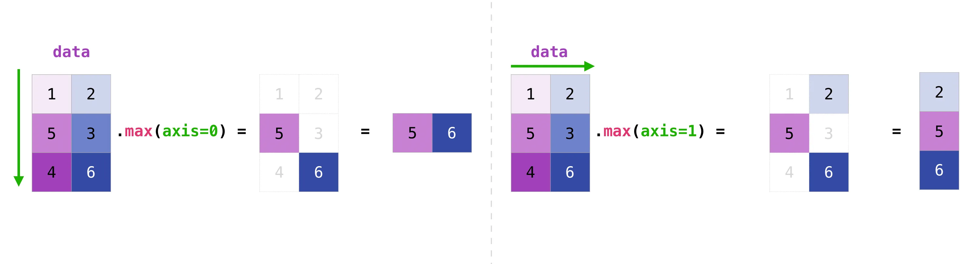
Think of axis=0 as “collapse the rows, leave the columns” and axis=1 as “collapse the columns, leave the rows”.
Four patients had their blood glucose measured (mg/dL) three times a day (morning, afternoon, evening):
data = [ [ 95, 105, 99], # patient 1 [ 89, 112, 102], # patient 2 [110, 129, 115], # patient 3 [100, 108, 104], # patient 4]Write a program that:
- stores the data in a NumPy array using the smallest dtype that fits all values,
- prints the shape and total memory used (
nbytes), - prints the readings of the last patient,
- prints the morning readings of every patient,
- prints the average glucose per patient.
All values are between 89 and 129, which fits comfortably in a signed 8-bit integer (range −128…127), but int16 is a safer choice if any reading could exceed 127.
import numpy as np
data = np.array([    [ 95, 105,  99],    [ 89, 112, 102],    [110, 129, 115],    [100, 108, 104],], dtype=np.int16)
print("shape:", data.shape)        # (4, 3)print("bytes:", data.nbytes)       # 24
print("last patient:", data[-1])print("morning:    ", data[:, 0])print("avg/patient:", data.mean(axis=1))
Sorting, concatenating, transposing, flipping
np.sort(np.array([2, 1, 5, 3]))# array([1, 2, 3, 5])
a = np.array([1, 2, 3])b = np.array([4, 5, 6])np.concatenate((a, b))# array([1, 2, 3, 4, 5, 6])
x = np.array([[1, 2], [3, 4]])y = np.array([[5, 6]])np.concatenate((x, y), axis=0)# array([[1, 2],#        [3, 4],#        [5, 6]])
transpose() (or .T) swaps axes:
a = np.arange(6).reshape(2, 3)# [[0 1 2]# [3 4 5]]a.T# [[0 3]# [1 4]# [2 5]]np.flip reverses an axis:
a = np.array([[1, 2, 3], [4, 5, 6]])np.flip(a) # reverse everythingnp.flip(a, axis=0) # reverse rows -> [[4 5 6] [1 2 3]]np.flip(a, axis=1) # reverse cols -> [[3 2 1] [6 5 4]]Adding and removing elements
When you change the size of an array, NumPy must allocate a new block of memory and copy the elements over — the original is left untouched.
That is why np.delete returns a new array:
a = np.array([[1, 2, 3, 4], [5, 6, 7, 8], [9, 10, 11, 12]])
a = np.delete(a, 1, axis=0)   # remove the second rowprint(a)# [[ 1  2  3  4]#  [ 9 10 11 12]]
np.append works similarly:
np.append(np.array([1, 2, 3]), [4, 5])# array([1, 2, 3, 4, 5])For frequent insertions or deletions, prefer Python lists or another data structure — every NumPy resize is a full copy.
Unique values
np.unique returns the sorted unique values of an array:
a = np.array([11, 11, 12, 13, 14, 15, 11])np.unique(a)# array([11, 12, 13, 14, 15])It can also return how many times each one appears:
values, counts = np.unique(a, return_counts=True)print(values) # [11 12 13 14 15]print(counts) # [3 1 1 1 1]You can use this to compute the mode (the most frequent value):
x = np.array([2, 2, 2, 3, 4, 4, 5, 5, 5, 5, 7])values, counts = np.unique(x, return_counts=True)mode = values[counts.argmax()]print(mode) # 5Missing data: NaN
When data is missing — a sensor failed, a survey question was skipped — you cannot leave a “hole” in a NumPy array, because every element must have a value. The convention for floats is np.nan (Not a Number), defined by the IEEE 754 standard.
arr = np.array([1.0, np.nan, 3.0, 4.0, np.nan])print(arr)# [ 1. nan 3. 4. nan]Any arithmetic involving nan propagates as nan — by design, because the result is undefined:
np.nan + 3 # nanarr.sum() # nanarr.max() # nanNumPy provides nan-aware variants that ignore the missing values:
np.nansum(arr) # 8.0np.nanmax(arr) # 4.0np.nanmean(arr) # 2.6666666666666665To find or count missing values, use np.isnan, which returns a boolean mask:
np.isnan(arr)# array([False,  True, False, False,  True])
np.isnan(arr).sum() # 2nan is not equal to itself: np.nan == np.nan is False. Always test for missing values with np.isnan(x), never with x == np.nan.
Saving and loading
For a quick interactive save, np.save / np.load use NumPy’s binary .npy format:
a = np.arange(10)np.save("data.npy", a)b = np.load("data.npy")For text data, np.savetxt / np.loadtxt work with CSV-like files:
a = np.array([[1, 2, 3], [4, 5, 6]])np.savetxt("data.csv", a, delimiter=",", fmt="%d")b = np.loadtxt("data.csv", delimiter=",")For real-world CSVs with headers and mixed columns, the pandas library is much more comfortable:
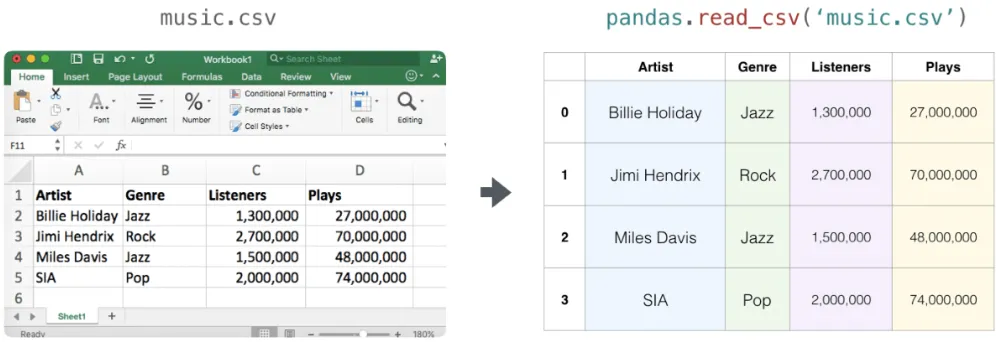
import pandas as pd
df = pd.read_csv("music.csv")arr = df.to_numpy()      # convert the DataFrame to a NumPy array
Practical example: production matrices
A car company has two factories — one in Spain and one in the UK — building two car models in three colours. The daily output of each factory is given by a 3×2 matrix.
Spain (matrix A) and UK (matrix B):
A = np.array([ [300, 95], [250, 100], [200, 100],])B = np.array([ [190, 90], [200, 100], [150, 80],])a) Total daily production:
total = A + B# [[490 185]# [450 200]# [350 180]]b) Spain raises production by 20%, UK lowers it by 10%. New total:
new_total = A * 1.2 + B * 0.9# [[531. 195.]# [480. 210.]# [375. 192.]]NumPy raises a ValueError if you try to add arrays of incompatible shapes — a useful safeguard against accidentally lining up the wrong data.
Practical example: Punnett squares
In genetics, a Punnett square shows every possible combination of two parents’ alleles. For two unlinked traits — coat colour (P dominant black, p recessive white) and tail length (C long, c short) — each parent contributes one of four gametes: PC, Pc, pC, pc.
The 4×4 grid of all combinations is:
import numpy as np
alleles = ["PC", "Pc", "pC", "pc"]square = np.empty((4, 4), dtype="U4")
for i, gi in enumerate(alleles):    for j, gj in enumerate(alleles):        # sort each gene's letters so PpCc and pPcC look identical        coat = "".join(sorted(gi[0] + gj[0], key=str.lower))        tail = "".join(sorted(gi[1] + gj[1], key=str.lower))        square[i, j] = coat + tail
print(square)
Now suppose we want the probability that an offspring is white-coated and long-tailed (ppCC, ppCc or ppcC):
flat = square.flatten()target = np.isin(flat, ["ppCC", "ppCc", "ppcC"])probability = target.sum() / flat.sizeprint(f"P(white & long tail) = {probability:.2%}")Practice
Given a 1D array of 12 monthly temperatures, reshape it into a (2, 2, 3) array — that is, two “halves of the year”, each split into two rows of three months.
temperatures = np.array([ 29.3, 42.1, 18.8, 16.1, 38.0, 12.5, 12.6, 49.9, 38.6, 31.3, 9.2, 22.2,])The trick is that temperatures.reshape(...) returns a new array — it does not change temperatures in place.
quarters = temperatures.reshape(2, 2, 3)print(quarters)print(quarters.shape) # (2, 2, 3)Use np.random.default_rng() to generate:
- an array with the ages of 10 students (each at least 16),
- an array of 10 blood types chosen at random from
["A+", "A-", "B+", "B-", "AB+", "AB-", "O+", "O-"].
Then append three older students (ages 35, 40, 45 with any blood types you like) and print both arrays.
import numpy as np
rng = np.random.default_rng()blood_types = np.array(["A+", "A-", "B+", "B-", "AB+", "AB-", "O+", "O-"])
ages = rng.integers(16, 31, size=10)groups = rng.choice(blood_types, size=10)
ages = np.append(ages, [35, 40, 45])groups = np.append(groups, ["A+", "B-", "O+"])
print("ages:  ", ages)print("groups:", groups)
rng.choice picks values uniformly from the given array. np.append returns a new array — it does not extend the old one in place.
You have students’ grades for two subjects across two terms:
term1 = np.array([ [7.5, 8.0], [6.0, 7.5], [8.5, 9.0],])term2 = np.array([ [8.0, 5.5], [4.0, 8.0], [9.0, 9.5],])Compute:
- the sum of grades per student per subject,
- boost the last student’s totals by 10%,
- the per-subject average of the first subject (column 0).
total = term1 + term2total[-1] *= 1.1print("total:", total)
avg_first_subject = total[:, 0].mean()print(f"avg first subject: {avg_first_subject:.2f}")Download a CSV with the average monthly temperatures of Barcelona from 2014 to 2023 (one row per year, twelve columns, plus a header):
Year,Jan,Feb,Mar,Apr,May,Jun,Jul,Aug,Sep,Oct,Nov,Dec2014,9.8,10.1,12.3,15.3,16.2,21.7,22.6,23.0,22.0,19.6,13.6,9.12015,9.1,8.2,12.0,14.8,19.1,23.2,26.0,23.5,19.7,16.7,14.3,12.6...2023,9.2,10.3,14.1,16.1,18.1,23.4,25.5,26.0,23.2,20.2,14.8,12.1Save the file as barcelona.csv. Then:
- load only the twelve temperature columns into a 2D array (skip the year column and the header),
- print the average temperature per year,
- print the hottest and coldest month each year.
import numpy as np
data = np.loadtxt(    "barcelona.csv",    delimiter=",",    skiprows=1,    usecols=range(1, 13),   # drop the Year column)
print("avg per year:", data.mean(axis=1))print("max per year:", data.max(axis=1))print("min per year:", data.min(axis=1))
skiprows=1 skips the header. usecols=range(1, 13) reads only columns 1 to 12, dropping column 0 (the year).
Quick reference
| You want to… | Use |
|---|---|
| Build an array from a list | np.array([...]) |
| Build a fixed-size array of zeros | np.zeros(shape) |
| Build a range of numbers | np.arange, np.linspace |
| Reshape without copying | arr.reshape(...) |
| Get a copy of an array | arr.copy() |
| Filter by condition | arr[arr > 5] |
| Combine arrays | np.concatenate, np.stack |
| Reduce along an axis | arr.sum(axis=...), arr.mean(...) |
| Handle missing data | np.nansum, np.isnan |
| Random numbers | np.random.default_rng() |
| Save / load | np.save, np.load, np.loadtxt |